How to Use Spatial Data to Map Rivers and Roads in Tableau

Spatial data is becoming increasingly relevant in the world of data visualization, and is easier to use with Tableau than ever before. Personally, I know I look at a map at least once a day, whether it’s part of a data viz for a news article, driving directions, or searching for a coffee shop. Maps can be utilized for a myriad of purposes other than location services, such as showing population, political or environmental trends.

In this post, I will show you how to get the most out of maps by connecting to spatial data, mapping rivers, creating buffers, and more.

View / Interact / Download

How To Use Distance And Buffer Calculations In Tableau

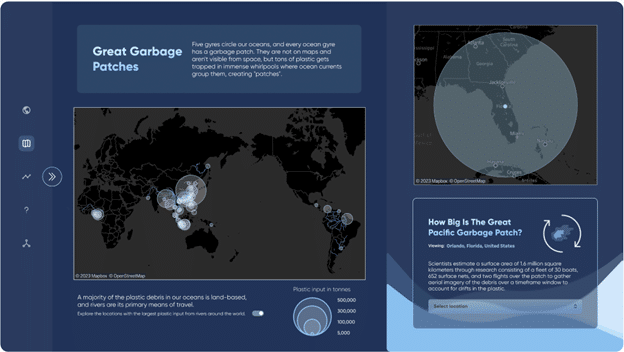
Last year, I utilized spatial data in our portfolio piece, “The Problem With Plastic,” to visualize the magnitude and location of plastic inputs from rivers in oceans by layering two separate spatial data sources on a single view. By creating multiple map layers, I was able to overlay one data source containing measurements of plastic inputs with corresponding latitude and longitude values over a shapefile of major world rivers in order to see which rivers were responsible for the largest plastic inputs.

View / Interact / Download

Spatial data doesn’t have to involve rivers (spatial lines); it can also feature points or polygons (states, counties, or any enclosed shape). Even so, in this tutorial, I am going to walk you through the steps for using spatial data to map rivers in Tableau, and how to implement the INTERSECTS and BUFFER functions as a bonus.

Connecting to spatial data in Tableau

Tableau can connect to a handful of spatial data types, including Shapefiles, MapInfo tables, KML files, GeoJSON, TopoJSON, and Esri Geodatabases. This tutorial will only focus on Shapefiles as a spatial data source.

Live Tableau Training
May 14 – 17, 2024

Learn directly from industry-leading experts, access hundreds of post-training resources, and more.

Book Your Spot

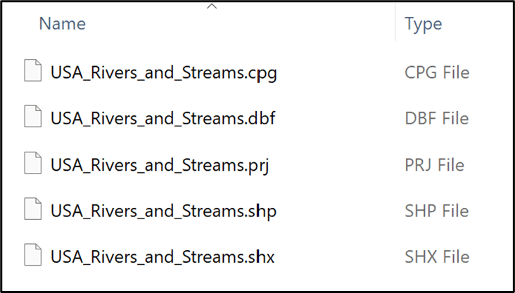
First, I suggest downloading this shapefile of USA Rivers and Streams from Esri Data and Maps to follow along.

Note: When you download a shapefile, it should download as a zipped folder containing multiple different file types. The zipped folder must contain these four file types: .shp, .shx, .dbf, and .prj, but some sources include other files with additional data. If you are curious to see the types of data included in this shapefile, you can unzip the folder, but make sure you select the zipped folder when connecting through Tableau.

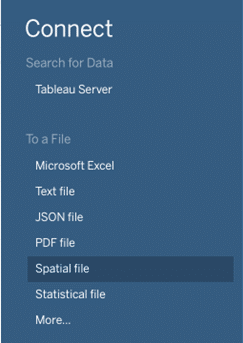
After downloading this file, you can open a new Tableau workbook, click Connect to Data and select Spatial file.

Mapping rivers with spatial data in Tableau

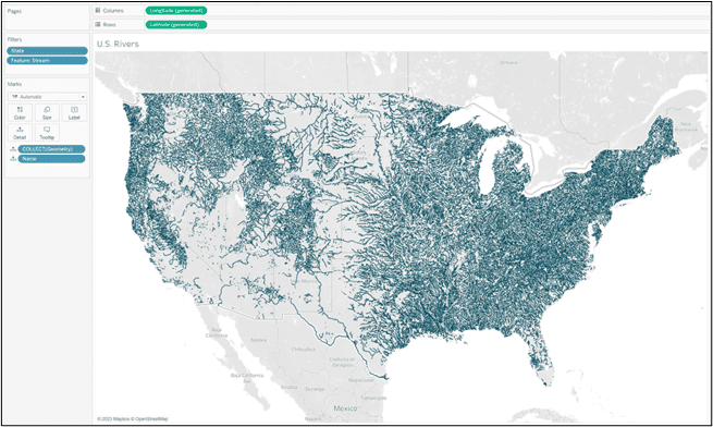
Once you have connected to the USA_Rivers_and_Streams data source, open up the first sheet in your workbook, and double-click on the “Geometry” field in your left Data pane. Tableau will recognize this as a “Map” mark type, and all of the rivers included in the data source should appear in your view.

By default, the rivers are connected as one single mark. (If you hover over any river segment, all of the rivers will highlight). To separate the rivers, drag an identifying dimension (“Name” in this case) to Detail on the Marks card. Now you should notice individual rivers are highlighted when you hover over the map.

Note, if any rivers have the same name, they will remain connected, and all segments will highlight when you hover over any river with that name. Some of the rivers are unnamed in this source, so you will notice they are still connected.

On the Marks card, select Color to adjust the opacity and color and set the Border and Halo options to None. Select Size and move the slider almost all the way to the left, around ⅛ of the bar.

Now you have successfully mapped rivers! You can filter your view like any other chart by dragging a dimension pill (e.g. Name, State, Feature) to the Filters shelf, and limit the number of rivers visible on your map. I filtered the view to only show Streams within the continental U.S.

How to use INTERSECT to find closest rivers to you

This map doesn’t tell us anything other than the location of rivers in the U.S., so we can add an additional data source to make the dashboard more informative. We are going to use the INTERSECT function introduced with Tableau 2022.4, and create a dashboard that shows rivers within a specific radius from Playfair’s Orlando and Kansas City offices.

Intersect spatial join

First, I used Google Maps to find the latitude and longitude of Playfair’s two offices and created a secondary data source, “Locations” with the following columns: City, State, Lat, Lng. Feel free to substitute any locations you want to map, or download my data source as a template.

Next, open the “USA_Rivers_and_Streams” dataset by clicking “Data Source” in the bottom left corner of the screen. Add a connection and select the new secondary data source, “Locations.” We are adding this new connection to the existing river data source, not creating a new data source. Double click “USA_Rivers_and_Streams” to open the physical table, and drag “Sheet1” from “Locations” onto the view to create a Join.

Related post: 3 Ways to Make Magnificent Maps in Tableau

We can perform an intersect spatial join between “USA_Rivers_and_Streams” and “Locations,” but we need at least one spatial polygon for this to work. Currently, we only have spatial lines (rivers) and spatial points (cities/addresses), but we can turn the points into polygons using the BUFFER function.

This function creates a boundary (or buffer) around a spatial point using your specified radius value and measurement (km, mi, ft, etc.), turning your spatial point into a spatial polygon.

How to Use Distance and Buffer Calculations in Tableau

Once you have opened the physical table, you can select the fields to join. On the left, select the “Geometry” field, then select “Intersects” as the join operator.

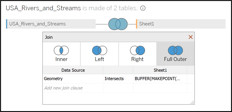
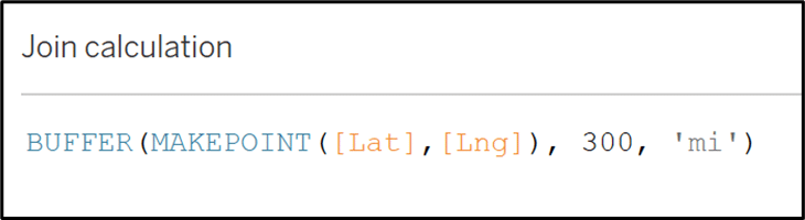
On the right under “Sheet1,” select “Create Join Calculation” and enter the below formula:

BUFFER(MAKEPOINT([Lat],[Lng]), 300, ‘mi’)

I chose 300 miles as an arbitrary buffer radius, and Full Outer Join so we can still see all of the rivers, not only ones within 300 miles of each office location. Note, the buffer radius can be adjusted to fit your personal use case, and if you want to filter out data not intersecting the Buffer you can use an Inner Join.

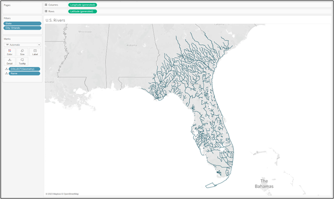
Your existing river map should not change after adding this spatial join, but now if you add “City” as a filter you will only see rivers within 300 miles of your selected city.

Creating points, buffers, and parameters

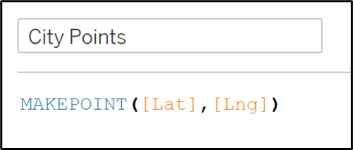
Now that we have the spatial join set up, we need to make a few calculated fields and parameters. First, remove all filters and use the following calculation to create spatial points for the two office locations:

MAKEPOINT([Lat], [Lng])

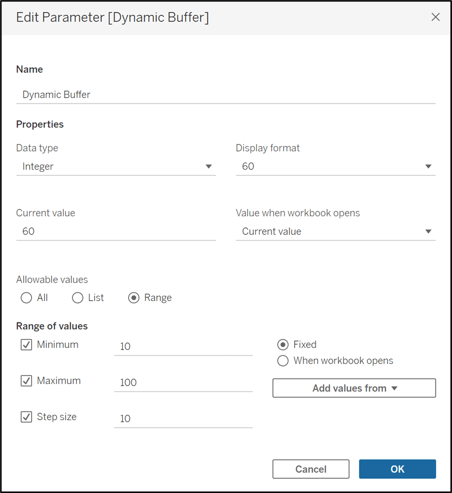
Next, create a parameter for a dynamic buffer we will use on our dashboard to choose the desired buffer/intersection radius (in miles). Make this parameter a range of integer values with a relevant min/max. I chose Minimum = 10, Maximum = 100, Step Size = 10.

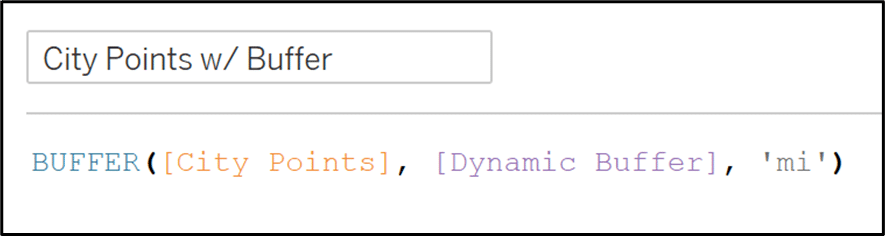
Now we can use this parameter in a calculated field to create spatial polygons centered on the City Points:

BUFFER([City Points], [Dynamic Buffer], ‘mi’)

Later on once this is mapped, you will see the size change with the parameter selection.

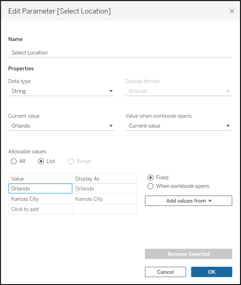
The second parameter we need to make is for location selection. It should contain the two cities in the “Locations” dataset, Orlando and Kansas City.

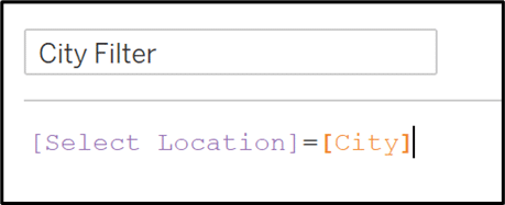
And now, create a calculated field we will use as a filter for this location parameter:

[Select Location]=[City]

Adding marks layers

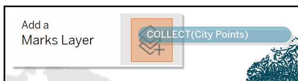
At this point, you can start adding additional layers to our existing river map. First, drag your calculated field “City Points” to the view and add it as a Marks Layer. The points won’t be very noticeable yet, as we haven’t filtered out any of the rivers or created an intersection filter.

I changed the Mark Type to Shape and used our Playfair Data logo as a custom shape, but you can use Circle, Square or any Shape as your preferred Mark Type.

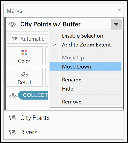
You also need to drag the second calculated field “City Points w/ Buffer” to the view as a third Marks Layer. Click the down arrow by the mark name, and select “Move Down” until it is below “Rivers.” Notice I renamed the original rivers Marks Layer from “Geometry” to “Rivers” to avoid confusion, and will also rename this Marks Layer from “City Points w/ Buffer” to “Selected City.”

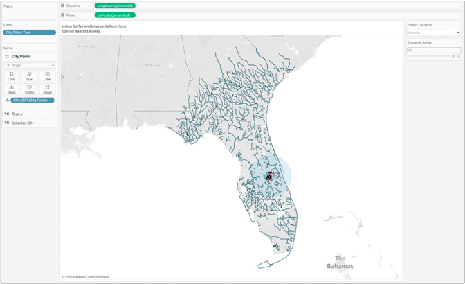
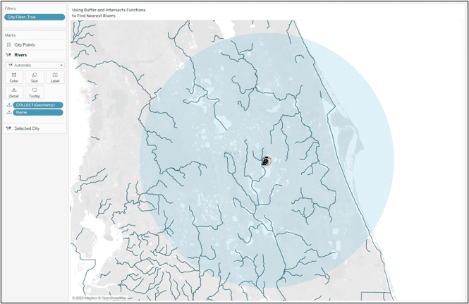
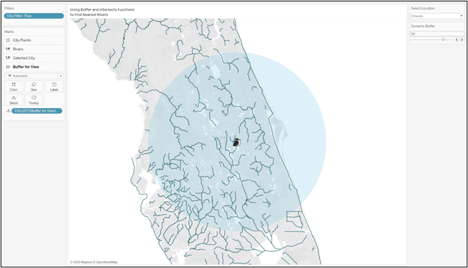
Now it is time to drag the calculated field “City Filter” to the Filters shelf and select “True,” and add both parameters to the view by right-clicking each parameter pill and selecting “Show Parameter.” You can adjust the color and opacity of the “Selected City” Mark, but note the size will not change since it is dependent on the parameter selection. Your view should now look similar to this:

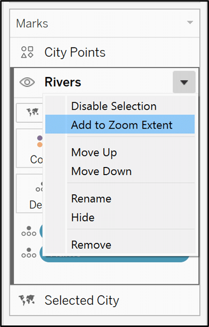
We want our view to be more cropped-in, so click on the “Rivers” Marks card, select the down arrow and make sure “Add to Zoom Extent” is NOT selected. This will focus our map around the buffer.

Now, your view should look like this:

Personally, I like a happy medium between the full view and cropped view so I created one more (optional) calculated field to add as a Marks layer. This adds an additional buffer to the parameter selection.

BUFFER([City Points], [Dynamic Buffer]+20, ‘mi’)

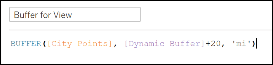
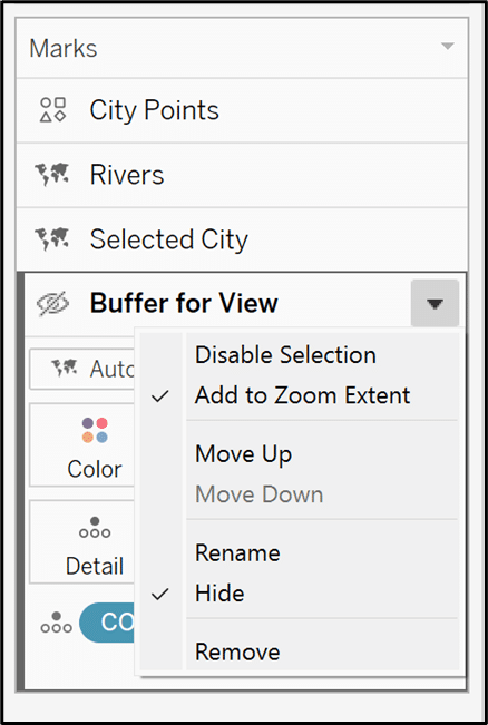
The color and mark types do not matter, because we can select “Hide” on the Marks drop down but keep “Add to Zoom Extent” selected. Now the map will zoom out to include this additional buffer, but not actually show the mark on the map.

I prefer this option because you can see more of the state and get better context from your map, but it is not necessary.

Using INTERSECTS function

Finally, the last step is creating an intersection filter with the following calculated field:

INTERSECTS([City Points w/ Buffer], [Geometry])

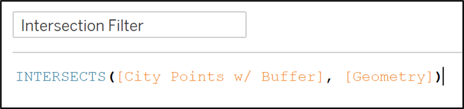
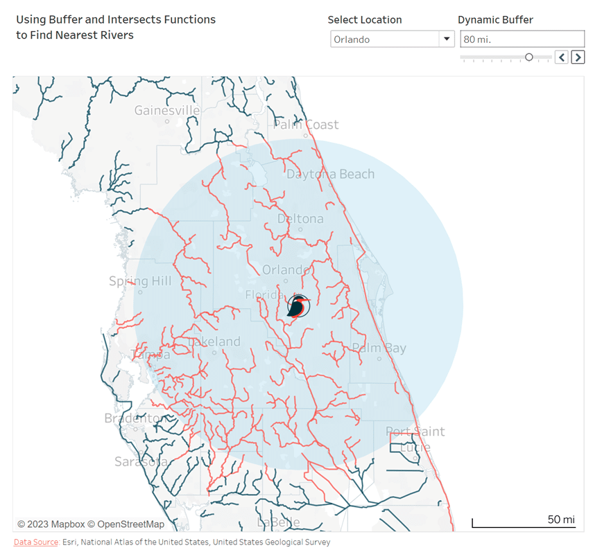
This calculation will return TRUE if any part of a river (Geometry) intersects with the selected city and buffer (City Points w/ Buffer).

Receive More Free Data Tutorials Like This Every Week

Let’s stay in touch:

Email(Required)

Δ

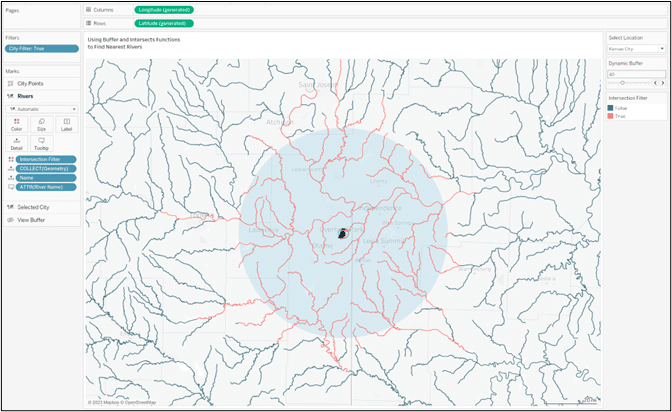
Drag “Intersection Filter” to the Color property of the “Rivers” Marks card, and voila! The rivers falling within your selected city buffer should be highlighted and will update with parameter selections.

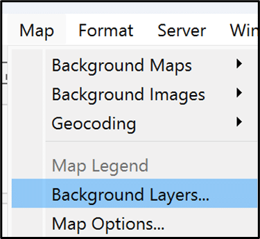
As a final touch, you can customize your map by clicking “Map” on the top toolbar and selecting “Background Layers” to edit the background map, or “Map Options” to show/hide map controls and add a scale legend. Update tooltips to your preference, and don’t forget to cite your data source if necessary!

Thanks for reading, and remember you can always find more spatial data files online to experiment with and create your own dashboard!

– Megan