Has there ever been a need to find, select, replace or format minor details of multiple cells in large datasets? Navigating through each cell to find the incorrect data can be extremely time-consuming and has a high potential for user error. I’ve recently encountered this challenge working with multiple large datasets, with unwanted merged and empty cells. Part of the data engineering process is to alleviate these inconsistencies, to make the data possible to work with. Attempting to go through each row and column is possible in a smaller dataset, albeit time-consuming – but what if you are presented with a large amount of data with thousands of rows? Surely, there must be another method. Luckily, Microsoft Excel is equipped to resolve this issue, maximizing your productivity and improving your final outputby utilizing the Go-To Special function with Microsoft Excel.

Go-To Special function with Excel: Merged cells

Enter: The Go-To Special function with Microsoft Excel

Not the easiest function to find in Excel, but definitely a useful tool to have in your kit. The Go-To Special function is a neat tool to quickly find and select cells based on what you’re searching for in your worksheet.

To find the Go To Special function:

• Open Microsoft Excel, then navigate to the Home tab in the ribbon.
• On the far right, there will be a category labeled Editing.
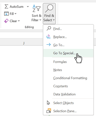
• The last option will be labeled Find & Select.
• Upon clicking on Find & Select, a dropdown menu will appear with Go To Special.

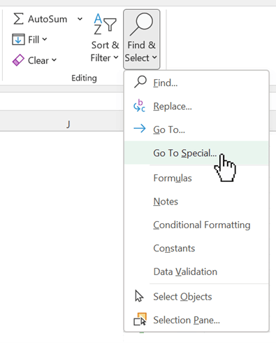
Upon clicking Go To Special, a pop up menu will appear with a myriad of options allowing you to select cells based on a specific criteria.

Live Tableau Training
May 14 – 17, 2024

Learn directly from industry-leading experts, access hundreds of post-training resources, and more.

Book Your Spot

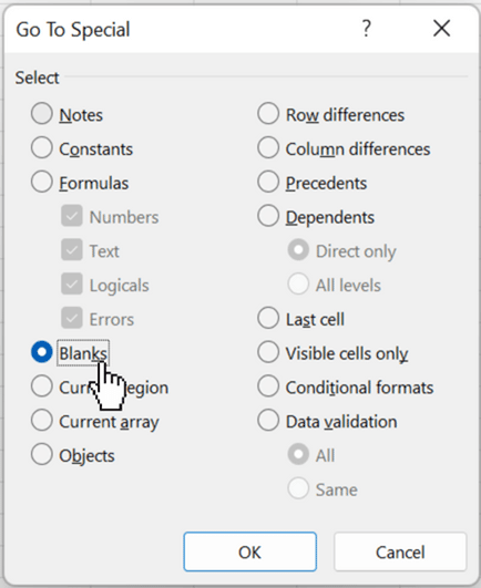
For this purpose, to identify the sneaky merged cells in a large dataset, select the Blanks option and click OK.

This will highlight every empty cell and merged cells (these are considered to be empty cells).

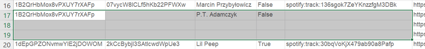
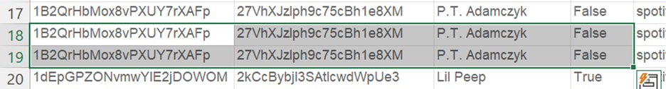
Please see below for an example using my extracted liked songs data from Spotify:

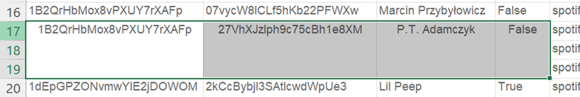
Let’s focus on the highlighted data. The data was merged by default as the three rows each have the same value, naturally, Microsoft Excel did this to make it easier for you to interpret.

However, this can be problematic for data engineering uses- so let’s get into unmerging these cells.

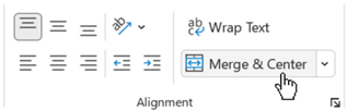
Navigate to the Alignment category in the ribbon and click Merge & Center to unmerge them.

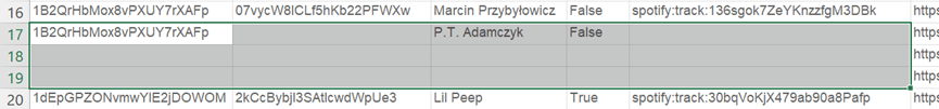
After unmerging the cells, it should resemble this, with the cells that were once merged, empty in their default positions:

Sweet! Your cells throughout your worksheet are now unmerged, your data may look a bit easier to work with now.

However, we’re not done just yet- let’s look into how to address those empty cells.

Empty cells

Your use cases for empty cells may vary, but it is likely that if they were previously merged then they share the same data as the cell it was merged to.

In the previous unmerging example, I liked three tracks from P.T. Adamczyk- these songs share the same values, so how do we populate these empty cells with those values without going through each cell and inputting the data?

Go-To Special has this functionality as well. It’s easy, I promise.

So, let’s get started.

First, navigate back to the Go To Special menu as mentioned above.

As expected, your pop-up will appear with the criteria you want to set. Select Blanks again. Remember, this will select the empty cells in your dataset. Click OK.

Once the empty cells are highlighted, navigate to the Formula Bar and input “=’ and the cell you wish to duplicate.

Receive More Free Data Tutorials Like This Every Week

Let’s stay in touch:

Email(Required)

Δ

See here for an example:

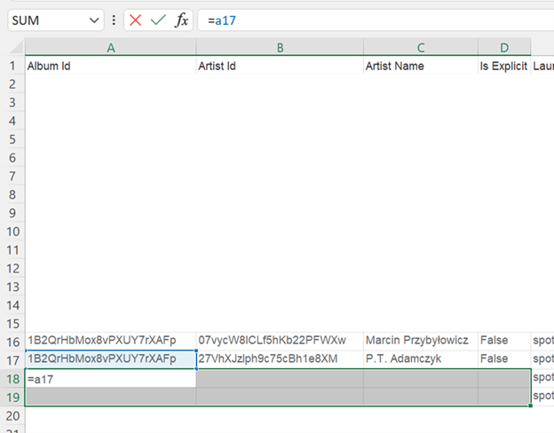
“A17” is entered in the formula bar as I want the values in row 17 to be duplicated to rows 18 and 19. Then, press Ctrl + Enter on your keyboard to have Microsoft Excel fill all selected cells with this formula.

Thus, all previously unmerged cells will be populated with the duplicated data.

With the cells that were merged, separated and populated with the correct data. You can attempt scrolling through your data to attempt to identify any discrepancies, it is unlikely that you will, but it is still worth checking.

And there you have it! An efficient way to clean your data using the Go-To Special function in Microsoft Excel.

That’s all folks!
Jaycii