An Introduction to the Power BI Power Query Editor

With the Power BI Power Query Editor, the data engineering world is at your fingertips. You can shape data to your heart’s (or report’s) content. In this tutorial we’ll dive into Power Query Editor and learn the basics of transforming your data. We’ll explore some data transformation options in the Home, Transform, and Add Columns ribbons with a simple use case.
FAQs answered in this post:
What is Power Query Editor and how do I access it in Power BI?
Power Query Editor is Power BI’s data transformation tool that allows you to shape and clean data before loading it into reports. Access it by clicking Transform Data in the Home ribbon of Power BI Desktop, or right-click any table in the Data pane and select Edit Query. The interface includes your queries list on the left, M formula language code in the middle, table preview below, and Applied Steps tracking all transformations on the right.
What is the difference between pivot and unpivot in Power Query?
Unpivoting transforms column headers into attribute-value pairs, converting wide data into tall data format ideal for analysis. This operation is found in the Transform ribbon and creates two columns: one for attributes (former column names) and one for values. Pivoting does the opposite, spreading attribute-value pairs back into separate columns, which is useful when you need to reshape normalized data for specific reporting requirements.
Should I rename columns using the interface or M code in Power Query?
Renaming columns directly in the M formula language is more efficient than double-clicking headers because it avoids creating additional Applied Steps. Each Applied Step increases query size and can slow down report load times, so editing M code to rename multiple columns simultaneously improves performance. This becomes particularly important in larger queries where minimizing steps accelerates refresh times and reduces memory consumption in enterprise deployments.
How do I create custom columns in Power Query Editor?
Navigate to the Add Column ribbon and click Custom Column, then write your formula referencing existing columns in square brackets like [Amount] / 34. Power Query also offers Column From Examples and Invoke Custom Function for more advanced scenarios. When deciding between Add Column and Transform ribbons, choose Add Column to create new columns and Transform to modify existing ones, as unnecessary columns increase query size and load times.
What are Applied Steps and why do they matter in Power Query?
Applied Steps is the step-by-step record of every transformation made to your data, displayed in the right pane of Power Query Editor. Each step generates M code that executes sequentially when refreshing data, so minimizing steps improves performance. You can click any step to see data at that point in the transformation, delete unnecessary steps, or edit step properties using the gear icon, making Applied Steps essential for troubleshooting and optimizing query efficiency.
How can Playfair Data help improve our Power BI data preparation workflows?
Playfair Data teaches Power BI engineering fundamentals including Power Query optimization, M formula language best practices, and efficient transformations that reduce load times. Our experts help organizations build scalable data pipelines using unpivot operations, custom columns, and Applied Steps management. Book a strategy call to learn how our Flagship Power BI workshops can help your team master data preparation techniques that improve report performance and stakeholder satisfaction.
Opening up Power BI Power Query Editor and creating a blank table
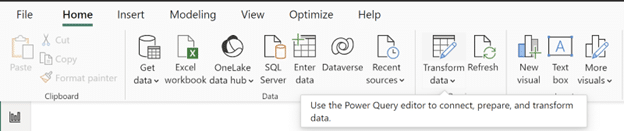
To get started, open up Power BI Desktop and click on ‘Transform data’ in the home ribbon.
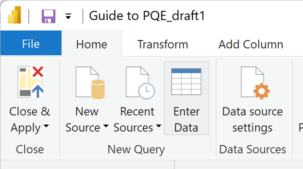
Now click on the New Source dropdown once the Power Query Editor window opens and click on Enter Data to create a new table. We’ll use this table to navigate through Power Query Editor.
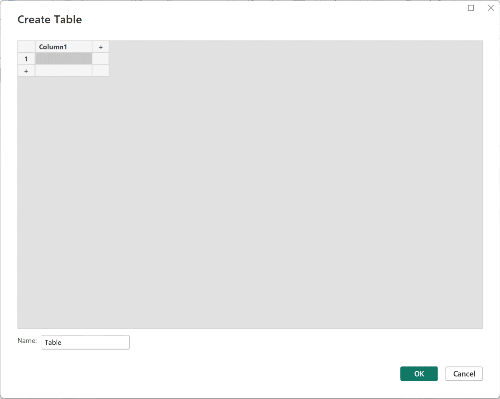
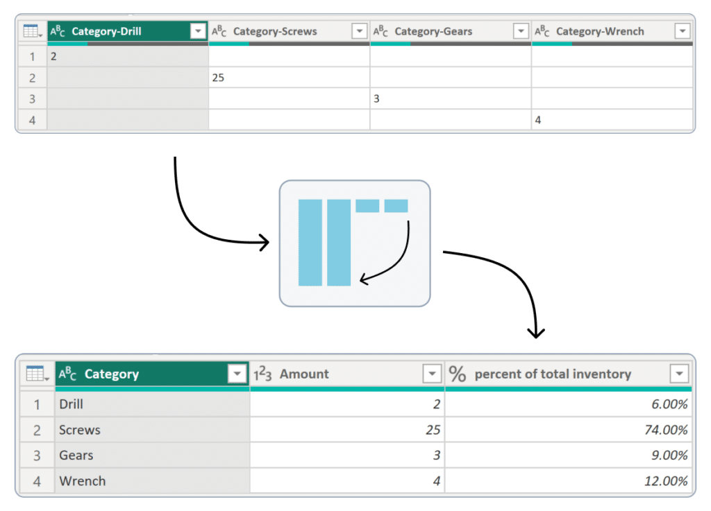
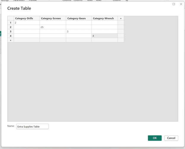
Name your table “Extra Supplies Table” and start writing. We want four columns (Drills, Screws, Gears, Wrench) and we want each column to start with “Category-” before the column name (Category-Drills, Category-Screws, Category-Gears, Category-Wrench). Enter values 2, 25, 3, and 4 along the diagonal. This is how your table should look at this point:
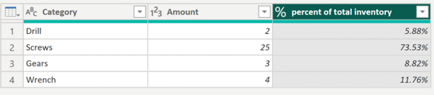
Now hit OK button in the bottom-right corner of the window to create the table. You should see your new table appear in the list of Queries on the left-hand side. Before we continue our tour, let’s establish a target for what we want this final table to look like after making some updates. Eventually, we want our table to look like the below image:
Now that we have a target in mind, let’s begin our tour of the Power Query Editor, starting with the PQE interface and the home tab.

Power Query Editor interface
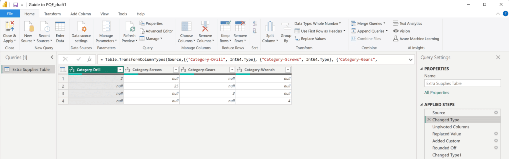
The PQE interface looks complicated, but it flows nicely. On the left you can see all of your loaded queries, the middle provides a block to edit the Power Query Editor’s data transformation coding language, called the M formula language, and a table view of your data in the selected query. The right-hand side shows all of the changes you make to any query, called “Applied Steps.”
The home ribbon gives you access to the most common and basic transformations like creating a table or blank query, adding or deleting columns and rows, changing column data types, and splitting columns. You can also merge and append queries.
Our current data structure is a bit inefficient and the structure and formatting doesn’t match our target table. To achieve the structure in our end table, we need to make use of the Transform ribbon.
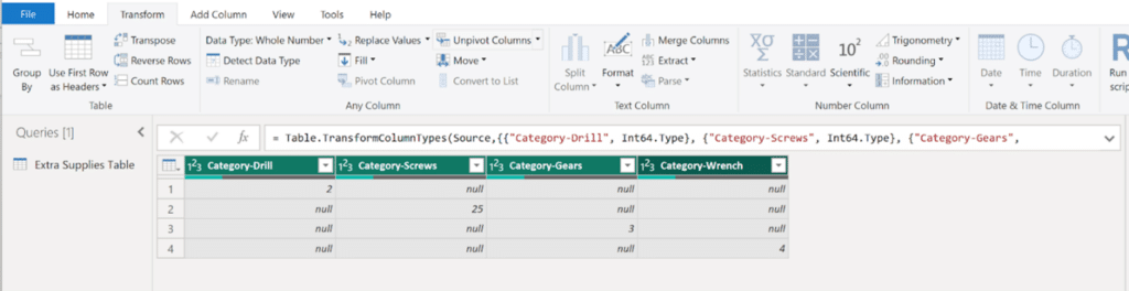
The Transform ribbon
The transform ribbon features some of the options from the Home ribbon as well as more complex column and row transformation options. Two of the most helpful options in the Transform ribbon are the ability to pivot and unpivot columns. These are essential in data transformation to achieve the data structure that you need.
Our first step in recreating our target table structure is to unpivot our data. This means that we want to transform the column (or columns) we want to unpivot from a column to an attribute-value pair. To do so, Shift-click on each of our four columns and click on Unpivot Columns. To see a brief description of the Unpivot Columns options, click on the dropdown arrow.
Once you unpivot the four columns, we are left with two columns.
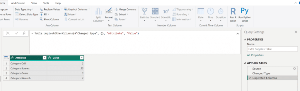
Notice the M code and the Applied Steps off to the right updating with every transformation we make. Now we’re left with our attribute value pairs! Our next order of business is to change our column names to Category and Amount, for which there are two approaches. Notice how our Applied Steps update differently with each technique.
How to Pivot, Unpivot, and Double Pivot Data in Tableau Prep
Approach #1: Double click on the column header, Attribute, to change the column name to “Category”.

Notice that with this first approach, we have a new Applied Step for the column we renamed. In a larger query, extra steps like these can increase query size which can increase load times, so I would recommend the following technique instead.
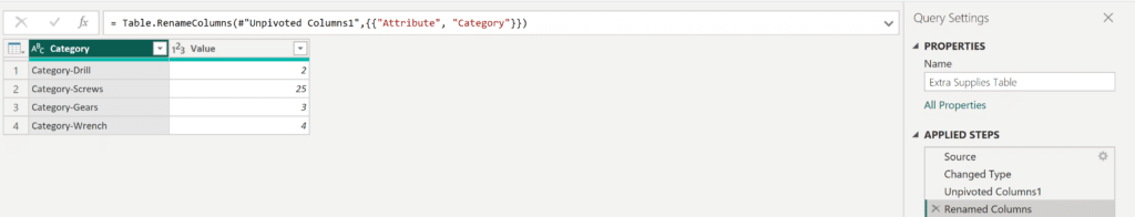
Approach #2: In the M code, replace “Attribute” with “Category” and “Value” with “Amount”, then hit Enter.
To achieve this second technique, we’ll have to go back to the previous step since we’ve only renamed the first column in the current step. In Applied Steps section on the right, click on the previous step. Now in the M code, replace “Attribute” with “Category” and “Value” with “Amount.”
Notice that we didn’t increase the number of steps in our query. Memory-saving tactics like these are essential to improving the load times of your Power BI reports. Now if you navigate back to the current step, Renamed Columns, we can see that the name of Column 2 was successfully updated. At this point, you’re safe to go ahead and delete the Renamed Columns step.
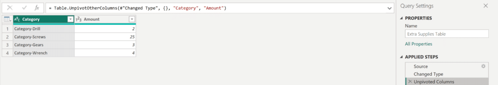
Now that we’ve got that sorted, we have no need for the preceding “Category-” in our first column. To update the names, start by clicking the Replace Values dropdown in the Transform ribbon.
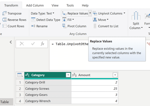
In the Value To Find box, enter “Category-” and leave the Replace With box blank.
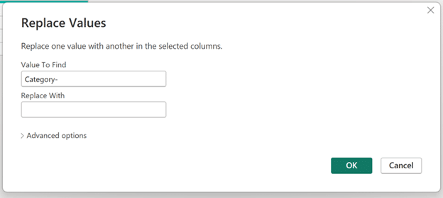
Now hit OK.
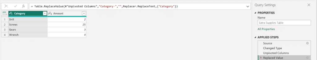
We have one new step representing the value we replaced and our Category column looks great.
Add Column Ribbon
To begin our next step in the Power BI Power Query Editor, we have to make use of the Add Column ribbon to create the % of Inventory column. Navigate to the Add Column ribbon by clicking on it from within the top navigation. Add Column provides you with the ability to perform all sorts of column transformations including extracting values from columns, parsing columns, formatting, using Date & Time, and the ability to perform many mathematical operations on your columns.
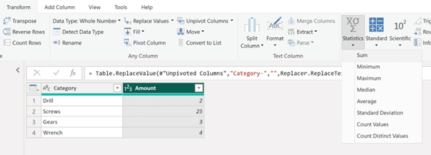
For this example, what we want is a new custom column that takes each Category and divides it by the total Amount of all categories. A quick way to find the sum of Amount is to go back to the Transform ribbon, click on the Amount column, click on the Statistics dropdown, and select Sum.
You should see a new step in Applied Steps and your screen should look like this.
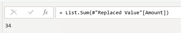
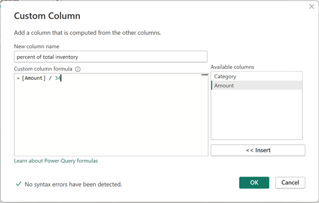
There are other ways to calculate column totals but since this is an introductory example, we’ll use this static value of 34 to create a custom column. Now that we have our value of 34, feel free to delete this step from Applied Steps. Now back in the Add Column ribbon, select Custom Column. In the popup dialog that appears, rename the column to percent of total inventory.
Continue reading with a free account, or login.
Unlock this tutorial and hundreds of other free visual analytics resources from our expert team.
Already have an account? Sign In
By continuing, you agree to our Terms of Use and Privacy Policy.
Now, in the Custom column formula box, double click on Amount from the Available columns section to the right and divide it by our sum of 34. The formula is = [Amount] / 34.
After hitting OK to confirm this, our Applied Steps updates and we have our newly-created custom column. I encourage you to continue exploring the custom column options as Column From Examples and Invoke Custom Function are very powerful tools.
Our last step is to round our new column and change the data type.
Before we continue, do we want to create a new column? Or would we like to not add any new columns? In this small example, the deciding factor is your preference. In a much larger query, most of the time it would be more efficient to avoid adding a new column. Why add a column and increase the size of your query/increase loading times if you don’t have to?
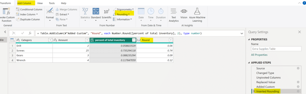
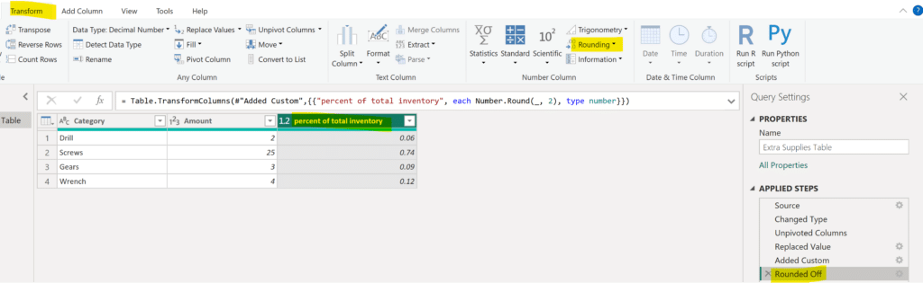
I bring this up because our answer determines which Rounding dropdown we select. If we select the Rounding dropdown in the Add Column ribbon, we will create a fourth column with the rounded values. If we select the Rounding dropdown in the Transform ribbon, we will round our third column and we won’t create a new column.
To round the new column by two decimal places, click on the Rounding dropdown in the Add Columns ribbon OR in the Transform ribbon and enter ‘2’ in the Decimal Places box. Hit OK to confirm the update.
Compare the two images below:
Changing data types
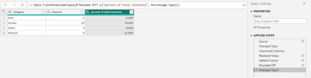
To change the data type from a decimal number to a percentage, we can change the data type from the Home, Transform, or Add Column ribbons. We can also change it by clicking on the Data Type box in our column.
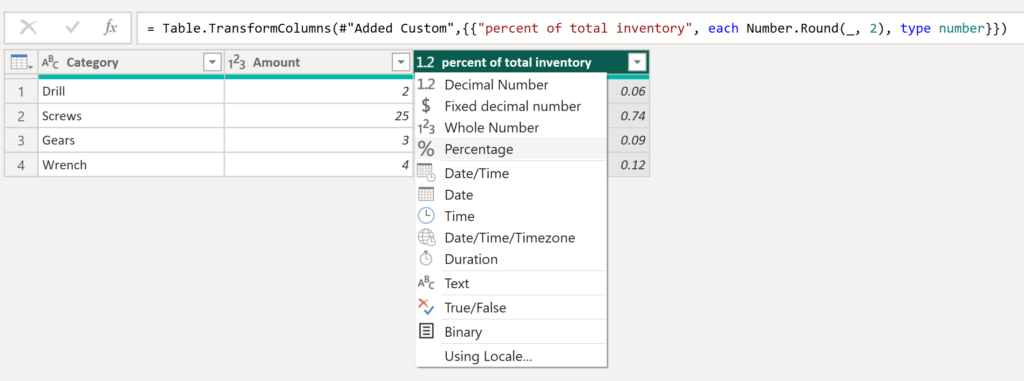
Change the data type to Percentage. Once again, our update is reflected in the Applied Steps section on the right. One last thing to note is that our percentages aren’t an exact match to our end goal table. To get closer to the exact number, just click the gear icon in the Rounded Off step and change the number of decimals!
And that’s it! We’ve matched our target table structure and used data transformation options from the Home, Transform, and Add Column ribbons in the Power BI Power Query Editor.
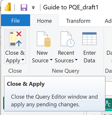
To apply our changes we’ve made, click on Close & Apply in the Home ribbon.
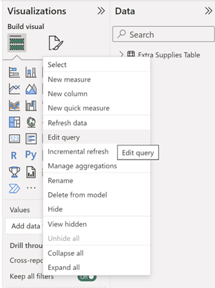
If you ever want to go back and make some changes to your data after you’ve already closed Power Query Editor and are in Power BI Desktop, simply right click on your table in the Data pane and click on Edit Query. Now we’re able to use our new, clean data to create impactful visuals and use our new column, Percent of Total, to compare inventory and use these numbers for analysis.
Thank you for reading,
Juan Carlos Guzman

Written By
Juan Carlos Guzman

Peer Review
Matt Snively
Sr. Manager, Analytics Engineering
Related Content
How to Connect to Data in Power BI Desktop
Microsoft’s Power BI is one of the top data visualization platforms on the market. The Power BI platform has products…
3 Ways to Make Beautiful Bar Charts in Power BI
Despite many new challengers over the years in the world of data visualization, bar charts have remained one of the…
3 Ways to Make Lovely Line Graphs in Power BI
If you read the first installation in this series on how to make Power BI bar charts more engaging, this…