Introducing Leapfrog Charts in Tableau

Leapfrog charts are a variation on a minimalist dot plot and can be used when the primary objective is to show the relative performance of a specific dimension member to a comparison point or points – or what it would take for that dimension member to ‘leapfrog’ over another, if you will. The dot plot is combined with a Gantt chart to illustrate the difference between a selected dimension member and a specific target or the average, median, minimum, or maximum for a measure across the business.

This chart was developed in conjunction with Playfair Data Information Designer, Jason Penrod. Keep reading to see how the chart looks and learn how to make it!

How to Make Leapfrog Charts in Tableau

Create a dot plot for the leapfrog chart

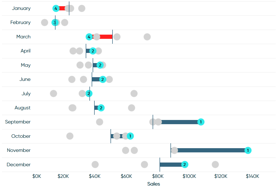
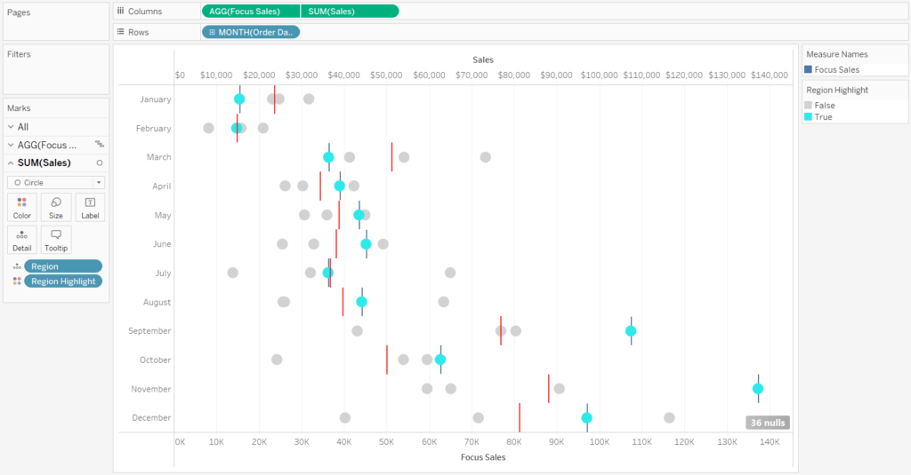
By the end of this post, you will be able to recreate the following chart. This example looks as Sales by Month by Region in the Sample – Superstore dataset and highlights the East region compared to the average for each month.

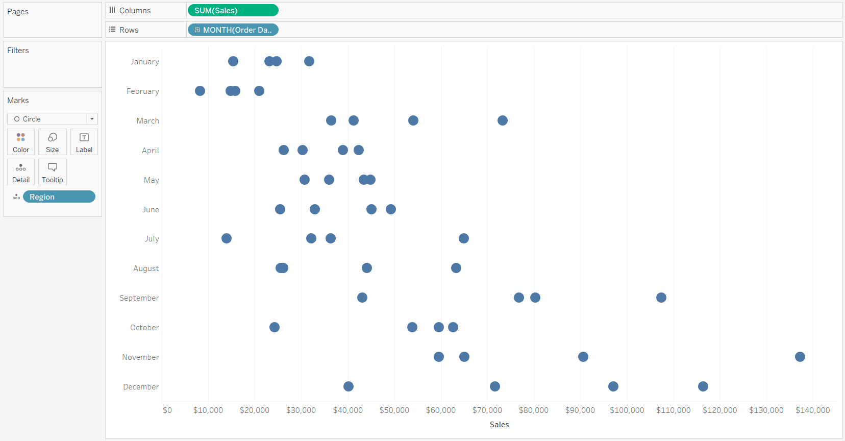
The first step to creating leapfrog charts in Tableau is to create the dot plot portion of the visualization. You can use any measure, any dimension to create the rows, and any dimension to create the circles, but for illustration, I will use Sales, Month of Order Date, and Region from the Sample – Superstore dataset, respectively.

New to Playfair Data?

Watch our 90-second intro video and receive tips on making your data usable.
 
Watch Video

To create the dot plot, place the measure on the Columns Shelf, the dimension that creates the rows on the Rows Shelf, change the mark type from Automatic to Circle, and place the dimension you want representing the circles on the Detail Marks Card.

Create the connecting Gantt marks

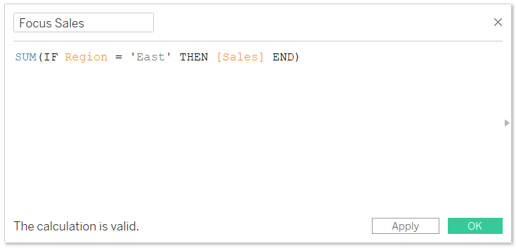
Now we need to create the Gantt chart that creates the bars in the background connecting the dimension member you are focusing on to the comparison point. In this example, I’m focusing on the East region and comparing its performance to the overall sales average per month. To get the Gantt mark in the appropriate place on the axis, you must isolate the performance for the dimension member being focused on with a calculated field.

One way to do this is to hardcode the dimension member of interest; the formula would be:

SUM(IF Region = ‘East’ THEN [Sales] END)

However, I suggest parameterizing the region selection so you can change the focus of the visualization on the fly. Here’s a Tableau tip within a Tableau tip; to create a parameter with a list of allowable values that matches the dimension members of a specific dimension, simply right-click on the dimension (i.e. Region) in the Dimensions area of the Data pane, hover over Create, and choose “Parameter…”. This will instantly create a parameter with the proper data type and your allowable values already populated.

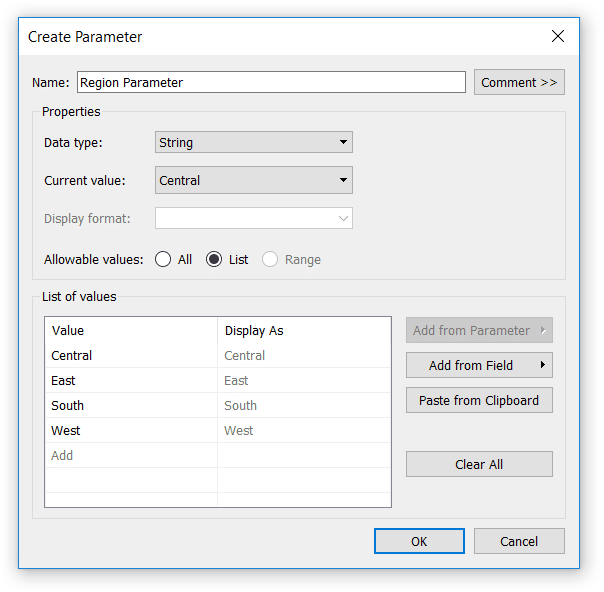
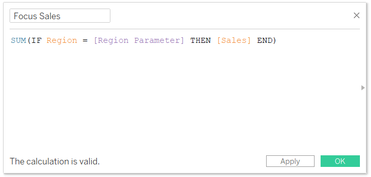
Note the default current value is the first allowable value, so I have switched that back to East to match the example in this post’s introduction. Now I will replace the hardcoded ‘East’ in the Focus Sales calculated field with this newly created parameter.

SUM(IF Region = [Region Parameter] THEN [Sales] END)

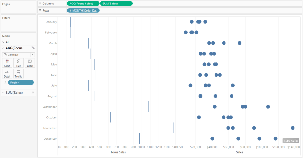
To use this calculated field to create the Gantt mark, place it on the Columns Shelf in front of the measure that is already there and change its mark type from Automatic to Gantt Bar. By placing the focus measure in front of the measure that was already on the Columns Shelf, it just ensures the Gantt marks are behind the circles in the final result.

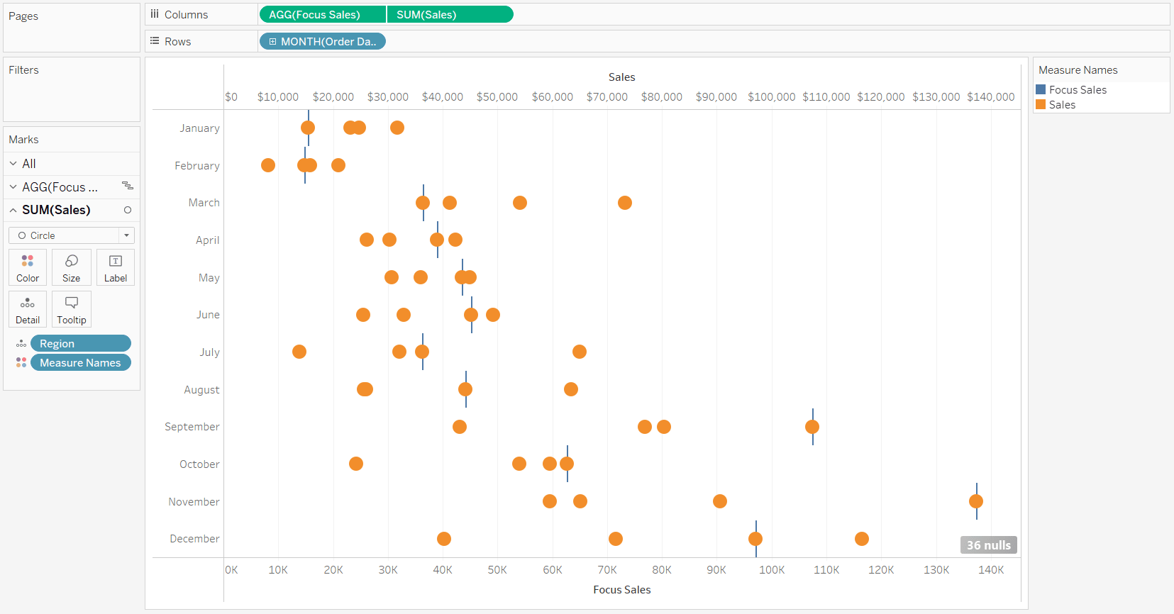
Convert this two-column chart into a dual-axis combination chart and ensure the axes are synchronized by right-clicking on either axis and choosing “Synchronize Axis”.

Add reference lines and highlights

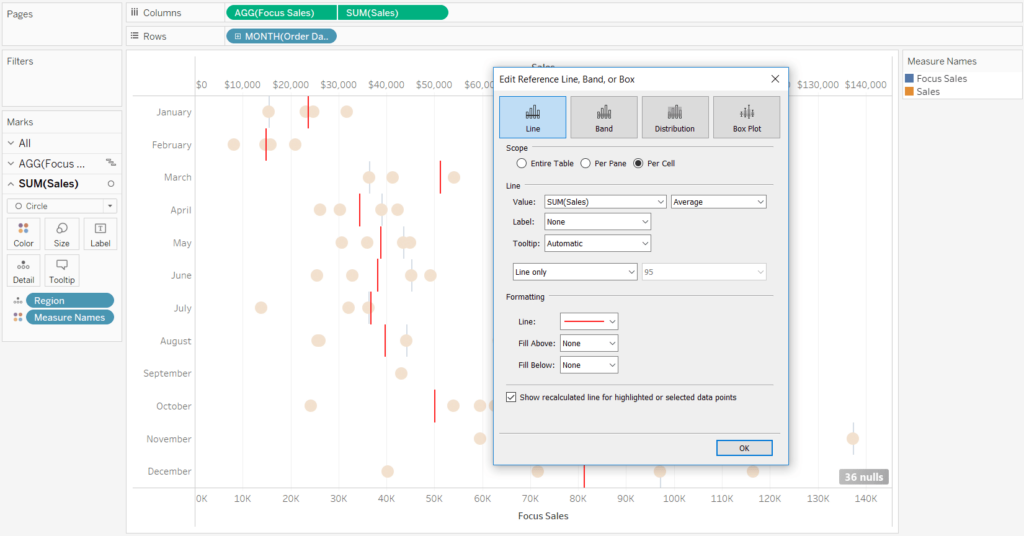
Since the comparison for this particular use case is average, I will go ahead and add a reference line for average per month to the Sales by Region axis. This will be helpful later when we quality check that the size and color of our Gantt marks are working as expected.

At this point, we have a circle for every region, a blue Gantt mark for the selected region, and a reference line showing us the average sales across all regions per month. Our focus region is starting to get lost, so I will create a calculation to color the focus region something different than the other regions. The most elegant way to write this calculation is:

[Region] = [Region Parameter]

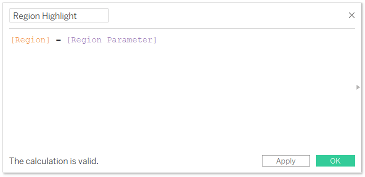
To create the highlight effect, replace the Measure Names field on the Color Marks Card of the dot plot with this newly created calculated field.

The Gantt marks need to be sized by the difference between the performance of your focus dimension member and the comparison, so we will need another calculated field. This is the calculated field that really makes this chart ‘go’. You can hardcode a target, isolate the performance of a benchmark, or as we’re doing in this use case, use window calculations to compare the dimension member to the average, median, minimum, or maximum for the measure being used.

Window table calculations are special in that they work across two axes, which we will need when using a dual-axis dot plot / Gantt chart. If I were wanting to compare the performance of the selected region to the average sales across sub-categories, the formula would be:

WINDOW_AVG(SUM([Sales])) – [Focus Sales]

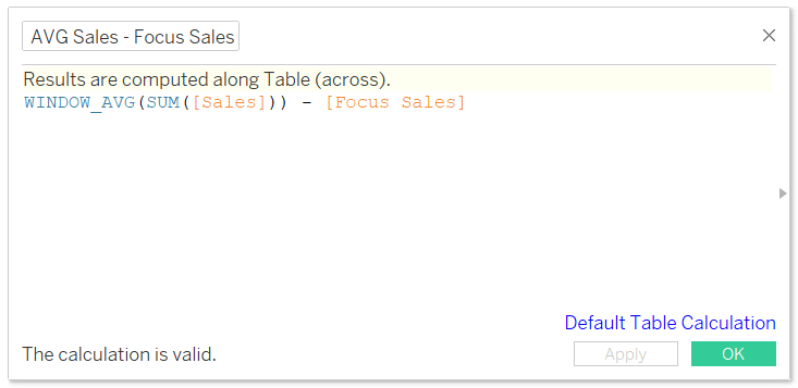
Place this calculated measure on the Size Marks Card for the axis drawing the Gantt chart.

By default, this table calculation is moving from the top of the table down, so while we are seeing the connecting lines come together, we need to change the addressing so that it includes the Region dimension and restarts the comparison every month.

An Introduction to Tableau Table Calculations

This can be a little tricky to get right but is helped significantly by using calculation assistance. You can change the addressing of a table calculation and see calculation assistance by right-clicking on the measure with the table calculation (currently on the Size Marks Card of the Gantt chart) and choosing “Edit Table Calculation…”. Note you can also reorder the dimensions in the table calculation by just dragging and dropping them in front of each other within this dialog box.

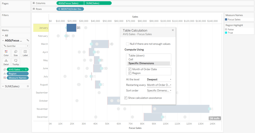
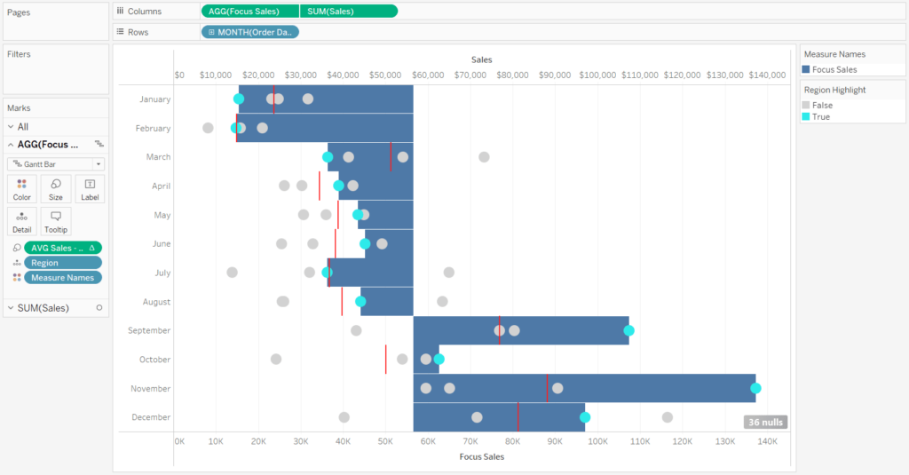
In this case, when the table calculation is updated properly, there should be a Gantt mark connecting the center of the focus dimension member and the average for each month.

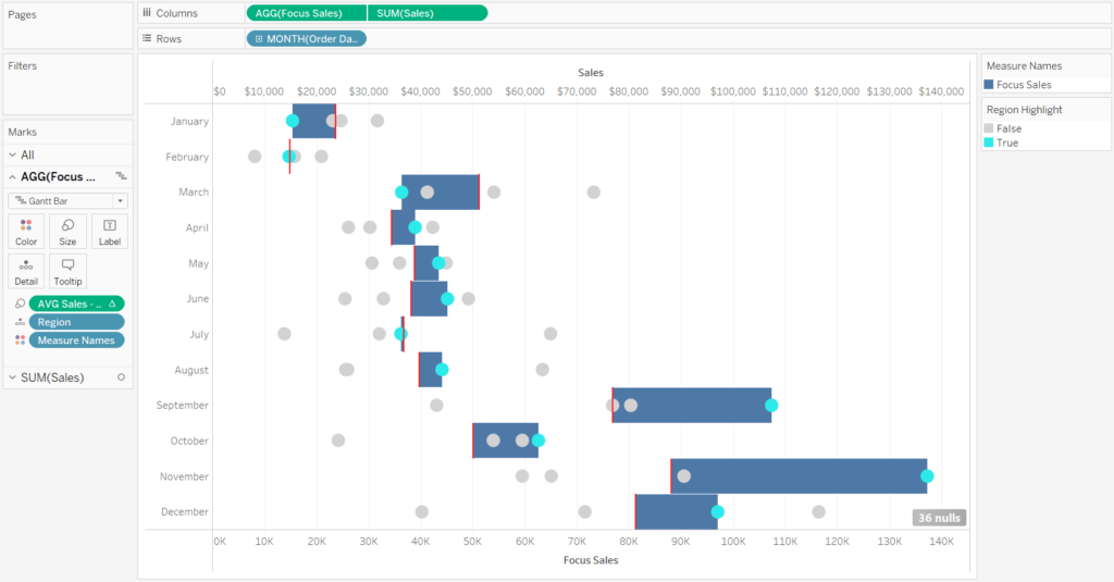
The Gantt mark should also be colored by this same calculation. The easiest way to do so is to navigate to the Marks Shelf for the Gantt Bar, hold the control key, and click on the measure containing the table calculation we set up during the last step while you drag it to the Color Marks Card.

By holding the Control key while clicking on a pill, it creates a duplicate of that pill, including any table calculations that may be applied. This is handy because we don’t have to edit the table calculation again to get the desired result.

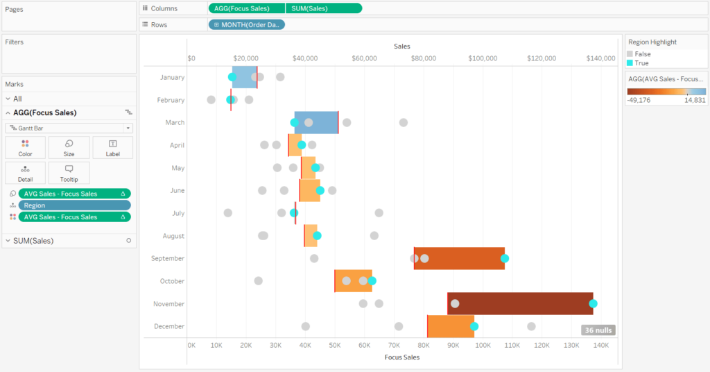
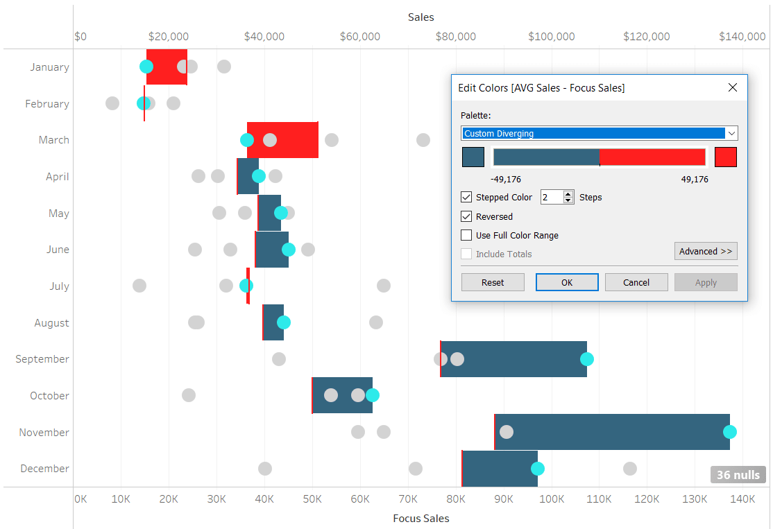
The Gantt bar colors don’t look quite right at this point because when my focus dimension member is past the comparison point, we should see a color that represents positive performance; otherwise we should see a color that represents negative performance. To flip the color scale and reduce the number of colors included in the spectrum, simply double-click on the color legend.

Finalize the leapfrog chart with formatting

From here, it’s all about the formatting. At a minimum, I recommend making the size of the Gantt marks skinnier and the circles slightly larger by clicking on their respective Marks Cards. I’ve also hidden one of the axes, hidden the indicators, turned off grid lines for Columns, changed the color of the reference lines, renamed the bottom axis, and put the fonts in brand.

At this point, we can already determine at a glance how the East region did compared to the comparison point of average sales per month. We can also see the contextual indicators of how it did versus the other regions in sales per month. One interesting insight is that the East region started the first three months of the year behind average, and not only passed the average in April, but widened its gap with the comparison as the year progressed.

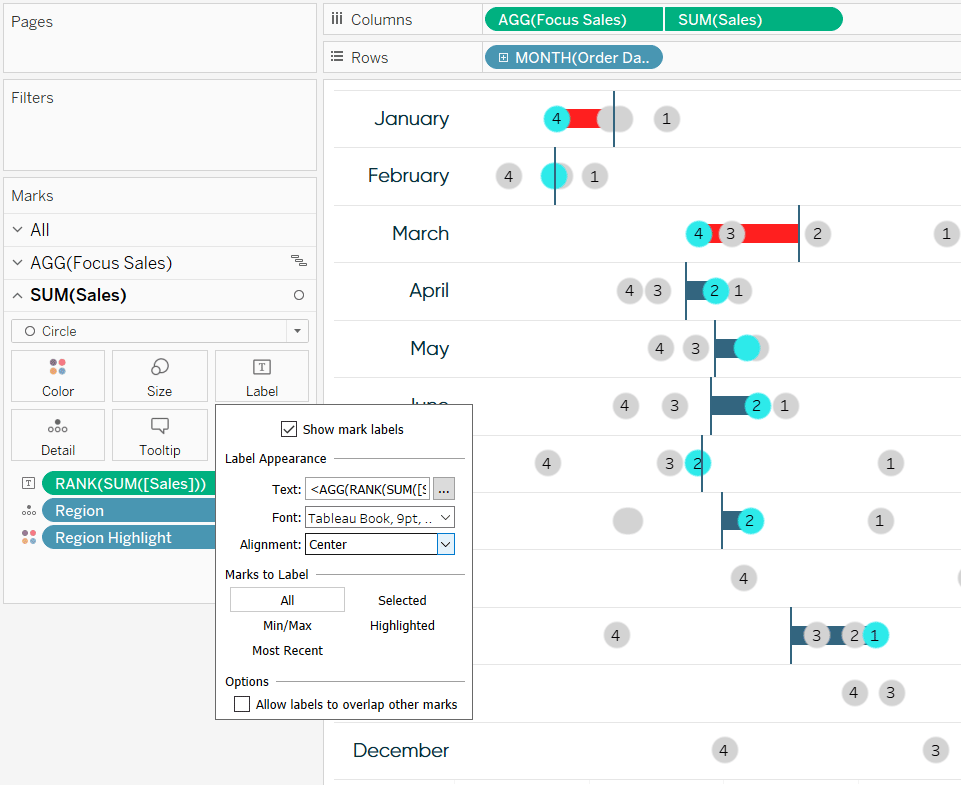
To add even more insight to this chart type, you can add a label to the circles that indicates rank. To do so, create a calculated field that computes the rank of SUM of Sales. This calculation can also be done in the flow directly on the Marks Shelf. In either case, the formula is RANK(SUM([Sales])) and should be added to the Label Marks Card.

Rank is another table calculation, so we need to ensure all the appropriate dimensions are being included, just as we did with the first table calculation above, for it to correctly compute the result. In this case, we want to see the sales rank computed across all our dimensions and restarting every month.

I will also center the labels on each circle by changing the settings on the Label Marks Card.

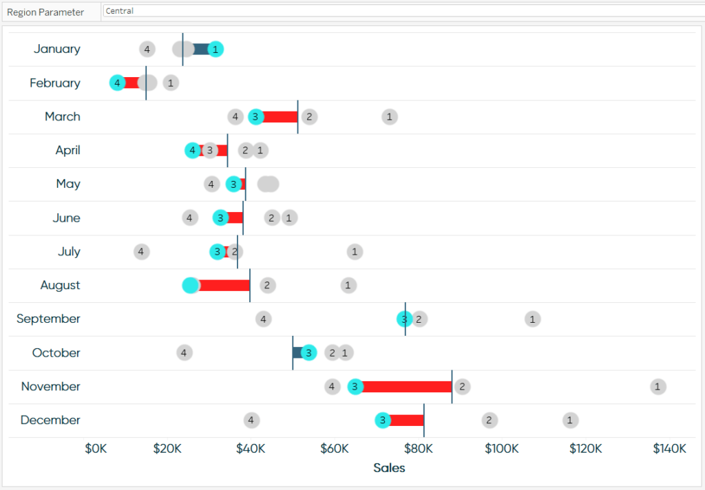
You have the option to only show the label for the focus dimension member as you saw in this post’s first image, but you will have more flexibility if you show all the labels. For example, because we parameterized the region selection, I can instantly change the focus of this visualization to the Central region and see a completely different story unfold.

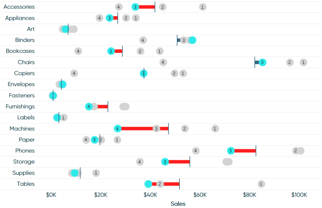
You can also change, or even parameterize, the dimension that is drawing the rows. However, you would have to update the table calculations to include the dimensional breakdown. Here’s how the view looks after replacing the Month of Order Date dimension with the Sub-Category dimension on the Rows Shelf.

Thanks for reading,
– Ryan